8. Statistics

The Coder allows some basic statistics to be performed, mainly descriptive statistics (reporting the means, etc., of each feature), and comparative statistics (splitting the codings into two or more sets, and reporting significant differences between these sets).

8.1 Descriptive Statistics

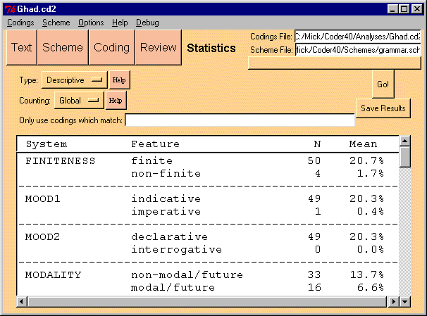
Selecting "Descriptive" in the Type field, and pressing the Go button will show the counts and mean value for each feature. You can also specify a filter to apply first, allowing you to get counts on subsets of the corpus. Filters are specified as in the Review section.

Figure 8: Descriptive Statistics

8.1.1 Local/Global Counting

This widget allows you to choose between two ways of deriving the mean:

Global Mean: The global mean represents the likelihood of selection in the corpus as a whole. It is derived by dividing the number of times the feature occurs in the codings by the total number of codings.

Local Mean: the local mean represents the likelihood of choice within a system. It is derived by diving the total number of codings with this feature by the total number of codings which select from the same system. Thus, the sum of means for all features in a system is always 100%.

The user can choose between these two modes using the popup menu on the interface.

8.1.2 Save Results

Pressing the Save Results button saves the results as plain text, or alternatively as an HTML file. This HTML file can be opened into MS Word as a way of getting the results into a report. For an example of results saved in HTML (using "Comparative: system-by-system) click here.

8.1.2 Exporting Data to Statistical Packages

For more detailed statistical analysis, the codings can be exported in a form (tab-delimited) which statistical packages can import. Choose "Save Codings As..." from the Codings menu, and change the File Type field to "Tab Delimited". The codings thus saved can be loaded in some statistical packages for more detailed analysis.

8.2 Comparative Statistics

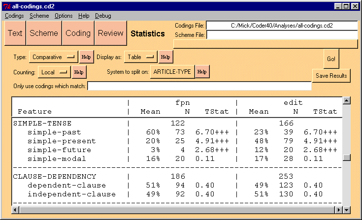
You can split your codings into two or more subsets and compare these subsets compare statistically. Choose "Comparative" in the Type field to start. See figure 8.

Figure 8: The Comparative Statistics Display

8.2.1 Setting up the Study

Selecting the Split System: You split your data on the basis of the features in a system. For instance, if you have a system: modal/nonmodal, then select this system in the "System to Split on" popup menu. The data will be split into two sets: codings with feature modal and codings with feature nonmodal.

Note: if you only wish to compare 2 features in a system with 2 or more features, use the following method.
i) Save your codings. ii) Go to the Scheme interface and delete the feature(s) you don't want in the comparison.
iii) Come back and do the statistical study. DO NOT SAVE THE CODINGS WITH THE DELETED FEATURE(S).

Filtering Data: You can use the filter to select only subsets of your data. For instance, you might wish to compare only finite-clauses. See the Review section for details.

Excluding Systems from the Comparison: if you don't want the comparison to include details on particular systems, you can i) return to the Scheme interface; ii) click on systems you want excluded iii) select "Ignore System". These systems will then be ignored in the statistical results.

Presentation in Table or Individual Systems: Using the "Display as" popup menu, you can choose to display the results as a table (see figure 8), or viewing an interpretation of the results system by system. Figure 9 shows the system-by-system method of presentation (actually from the results saved to html). Note that the Coder is here starting to write your report for you, doing some basic interpretation.

Note: Currently, system-by-system comparisons are only available for systems with two features. If you wish to compare between two features in a system with more features, use the Scheme interface to delete the excess features (BUT DON'T SAVE AFTERWARDS), then do the study.

System: REALIS

Feature	fpn(N=132)		edit(N=189)
	Mean	Stddv	Mean	Stddv	Tstat	Lvl
realis	0.720	0.451	0.598	0.492	2.259	++
irrealis	0.280	0.451	0.402	0.492	2.259	++

Interpretation

Set1 (fpn) exhibits significantly higher use of the feature: realis (72.00% vs. 59.80%).
Set2 (edit) exhibits significantly higher use of the feature: irrealis (40.20% vs. 28.00%).

Figure 9: System-by-System interpretation of comparison

Local vs. Global Counting: See Descriptive Statistics for the difference between these two ways of calculating means. In the context of comparative studies, you can choose to use local or global means as the basis of comparison.

Doing the Study: Once you have set all the options, press the "Go" button to have the study presented.

Saving the Study: Hit the "Save Results" button to save the study as either plain text or html.

8.2.2 Interpreting the Results: Significance & T-Statistics

The Table-mode presentation includes one column for each feature. The column provides the mean occurrence of the feature, the count of occurrences, and some information regarding how different this result is that for the other features.

The difference between means is shown in terms of two indicators:

Level of Significance: Firstly, at the end of the entry there will be between 0 and 3 "+" signs. These indicate how statistically significant is the difference of this features mean from that of the mean of all the other data put together:

(none) Not significantly different.
+ Significant at the 90% level (10% chance of error).
++ Significant at the 95% level (5% chance of error).
+++ Significant at the 98% level (2% chance of error).

The level of significance is important to establish how repeatable your results are. Results without significance may be accidents, and if we repeat the study with other texts, they might not be repeated. If results are highly significant they are likely to be repeatable if we apply the analysis to a totally different pair of texts. To understand this, a single + means that of any 10 results with one plus, you can expect one to be a false result (10% chance of error).

T-Statistic: T-Stats are the numbers on which the level of significance is derived. The bigger it is, the higher the level of significance, but this also depends on how much data you have. In some more scientific papers, you might be requested to provide T-Stats, but it is quite rare in linguistics. See textbooks on Statistics for more detail.

The System-By-System display also displays the standard deviation of each mean. This statistic tells you how much variation there is in your data. For more detail, see: see: http://www.robertniles.com/stats/stdev.shtml).

8.3 Comparing Two Files

You might wish to code two distinct texts using the same network, and then compare how they differ in their use of the systems. For instance, we might code an essay by a ten year old and one by a twelve year old and compare, or a corpus for Spanish and one for English. The Coder allows you to compare two files with the same network/scheme. To do this:

1. Ensure the two files use the same scheme when coding: As we have been working up to now, each file of codings has been saved with the coding scheme embedded in the file. The codings and the scheme are both in one file. However, another way of working is to have the scheme in a different file to the coding file. This means that several text files can share the same scheme. I call an external scheme a master scheme.

To convert from using a codings file with the scheme embedded to using an external master scheme: a) Open the Codings file. b) Under the Options menu, choose Save Options… c) In the presented window, choose Save to Master. d) Then press the Locate button in this window, and type in a filename for the new master scheme. Hit the OK button to return to the previous window, and press Done here.
The Codings file now requires this master scheme to be present whenever it is used. If you move it, the Coder will ask you to locate it.
When you Import Text to start a second codings file, you normally select "Start from Scratch" and build your own network afresh. This time, select "Use Master", and select the newly created Master scheme. You will then have to segment the new text, but you will have a scheme present already. So, after segmentation, you can move directly to coding.
Finish coding this second file, and save it to disk. If you change the network during this coding, you might want to re-open the first file, and update the codings to ensure that the changed network is ok for this file as well. In the Codings section, go to the first coding, and then press "Next Incomplete" to see if any need to be added to.

2. Open one of the files in the Coder.

3. Go to the Statistics interface, and select "Compare Files" from the menu which normally shows "Descriptive".

4. A new item appears on the screen, asking you to provide the filename to compare to: hit the Locate button and select another file which uses the same scheme.

5. Hit the Go button and the results should be shown.

8.4 Cell Analysis

This simple form of Cell Analysis finds all codings which have exactly the same features assigned to them. This is a useful tool to identify the recurrent patterns in your corpus. Select "Cell Analysis" from the "Type:" menu, and then press the "Go" button. The display will show each grouping, sorted by size.

For each group, it shows the features common to the group, and an example, the number of codings in the group, and the members of the group.

You can use "Ignore systems" in the Scheme window to reduce the number of systems used for cell grouping. Remove systems which are more delicate, or perhaps irrelevant for grouping.

Prior Section

Index

Next Section